Defining A Sensor Mask By Opposing Corners Example

This example demonstrates how to define a sensor mask using the grid coordinates of two opposing corners of a rectangle. It builds on the Homogeneous Propagation Medium and Using A Binary Sensor Mask examples.

Contents

Defining a sensor mask by opposing corners

In addition to the Cartesian and binary sensor masks used in the previous two examples, it is also possible to define a sensor mask using the grid coordinates of two opposing corners of a line (1D), rectangle (2D), or cuboid (3D). The recorded data is identical to that recorded using a binary sensor mask covering the same region, however, the output is indexed differently as discussed below. In 2D, the rectangular regions are specified as column vectors in the form [X1; Y1; X2; Y2], where (X1, Y1) and (X2, Y2) define two opposing corners of the desired rectangular sensor region in units of grid points, where (1, 1) defines the upper left corner of the grid. Multiple rectangles can be specified by adding additional column vectors to sensor.mask as shown below.

% define the first rectangular sensor region by specifying the location of
% opposing corners
rect1_x_start = 25;
rect1_y_start = 31;
rect1_x_end = 30;
rect1_y_end = 50;

% define the second rectangular sensor region by specifying the location of
% opposing corners
rect2_x_start = 71;
rect2_y_start = 81;
rect2_x_end = 80;
rect2_y_end = 90;

% assign the list of opposing corners to the sensor mask
sensor.mask = [rect1_x_start, rect1_y_start, rect1_x_end, rect1_y_end;...
               rect2_x_start, rect2_y_start, rect2_x_end, rect2_y_end].';

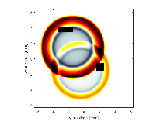
The computation is again started by calling kspaceFirstOrder2D. A snapshot of the simulation showing the two rectangular regions is given below.

Indexing the output data

When the sensor mask is defined using opposing corners, the output data is always returned as a structure (in the same way as when sensor.record is defined as discussed in the Recording The Particle Velocity Example). In this case, the recorded time-varying acoustic pressure is accessed as sensor_data(rect_num).p, where rect_num is the number of the rectangular region within sensor.mask. In this example, two rectangular regions are assigned to sensor.mask, so rect_num would be set to 1 or 2. As the shape of the sensor region is always regular, the output data is also indexed differently compared to using a Cartesian or binary sensor mask. In 2D, the sensor data is indexed sensor_data(x_index, y_index, time_index) (similarly in 1D and 3D). This makes it particularly useful for recording the results of a simulation in a plane or line without needing to reshape the output data. If the regions are overlapping, the overlapped data is returned as part of both sensor regions. An example of querying the size of the sensor data is shown below.

>> size(sensor_data(1).p)

ans =

     6    20   604

>> size(sensor_data(2).p)

ans =

    10    10   604