3D Time Reversal Reconstruction For A Spherical Sensor Example
This example demonstrates the use of k-Wave for the time-reversal reconstruction of a three-dimensional photoacoustic wave-field recorded over a spherical sensor.
The sensor data is simulated and then time-reversed using kspaceFirstOrder3D.
It builds on the 2D Time Reversal Reconstruction For A Circular Sensor and 3D Time Reversal Reconstruction For A Planar Sensor examples.
Contents
Simulating the sensor data
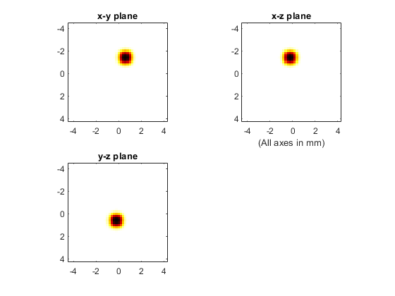
The sensor data is simulated using kspaceFirstOrder3D with an initial pressure distribution created using makeBall.
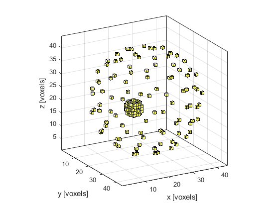
A Cartesian sensor mask of 100 points evenly distributed around a sphere (using the Golden Section Spiral method) is created using makeCartSphere.
A visualisation of the initial pressure and the sensor mask using cart2grid and voxelPlot is shown below.
Running the reconstruction
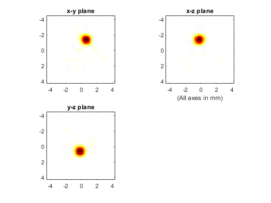
A plot of the initial pressure distribution and the reconstructed distribution using time-reversal are shown below (the three displayed image planes intersect at the centre of ball shown above). The plot scale for the reconstructed image has the plot limits reduced by a factor of 20.
Interpolating incomplete sensor data
The reconstruction can again be improved by interpolating the sensor data onto a continuous sensor surface. This is achieved using interpCartData and a binary sensor mask of a continuous sphere (created here using makeSphere) that is spatially equivalent to the Cartesian measurement grid. This function calculates the equivalent time-series at the sensor positions on the binary sensor mask from those on the Cartesian sensor mask via interpolation (nearest neighbour is used by default).
% create a binary sensor mask of an equivalent continuous sphere
pixel_radius = round(sensor_radius / kgrid_recon.dx);
binary_sensor_mask = makeSphere(kgrid_recon.Nx, kgrid_recon.Ny, kgrid_recon.Nz, pixel_radius);

% interpolate data to remove the gaps and assign to time reversal data
sensor.time_reversal_boundary_data = interpCartData(kgrid_recon, sensor_data, sensor_mask, binary_sensor_mask);
Details of the interpolation are printed to the command line.
Interpolating Cartesian sensor data...
  interpolation mode: nearest
  number of Cartesian sensor points: 100
  number of binary sensor points: 4234
  computation completed in 0.02934s
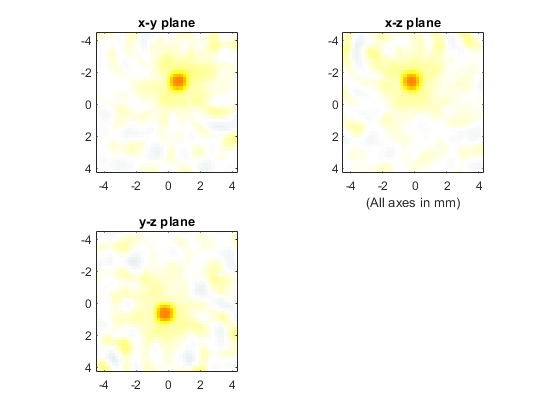
The reconstruction after interpolation is shown below. The plot limits are set to match those of the initial pressure plot shown above.