3D Time Reversal Reconstruction For A Planar Sensor Example

This example demonstrates the use of k-Wave for the reconstruction of a three-dimensional photoacoustic wave-field recorded over a planar array of sensor elements. The sensor data is simulated and then time-reversed using kspaceFirstOrder3D. It builds on the 3D FFT Reconstruction For A Planar Sensor and 2D Time Reversal Reconstruction For A Line Sensor examples.

Contents

Performing the reconstruction

The sensor data is simulated using kspaceFirstOrder3D in the same way as in preceding examples. The utilised initial pressure distribution and the sensor mask are shown in 3D FFT Reconstruction For A Planar Sensor. The time-reversal reconstruction is then performed by assigning the time varying pressure recorded over the detector array to sensor.time_reversal_boundary_data.

% run the simulation
sensor_data = kspaceFirstOrder3D(kgrid, medium, source, sensor, input_args{:});

% reset the initial pressure
source.p0 = 0;

% assign the time reversal data
sensor.time_reversal_boundary_data = sensor_data;

% run the time-reversal reconstruction
p0_recon = kspaceFirstOrder3D(kgrid, medium, source, sensor, input_args{:});

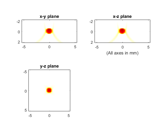
A plot of the reconstructed initial pressure distribution with a positivity condition is shown below.